class: center, middle, inverse, title-slide .title[ # The measurement of meaning from text ] .author[ ### David Garcia <br><br> <em>ETH Zurich</em> ] .date[ ### Social Data Science ] --- layout: true <div class="my-footer"><span>David Garcia - Social Data Science</span></div> --- # Outline ## 1. The semantic differential ## 2. Word embeddings --- ### Psycholinguistics: How individuals use and adopt language .center[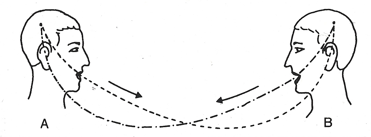] **De Saussure's model of language** - Language as association between signified (meaning) and signifier (word) - Associations are normative and agreed through learning - Human communication is composed of two steps: 1. **Encoding:** Transforming thoughts into words 2. **Decoding:** Translating words into thoughts --- # Connotative vs denotative meanings   - **Denotative meaning:** Definition of a word in reference to other meanings - **Connotative meaning:** Emotional association of the use of a word - Sentiment analysis aims to measure the **connotative meaning** of texts --- # The Semantic Differential **Charles Osgood's Semantic Differential:** Rating scales to measure the connotative meanings of words, objects, events (or symbols in general) Osgood's method to find the dimensions of meaning: 1. Select a set of objects/words/symbols to measure their meaning 2. Design a large set of questions or scales about the symbols 3. Ask some people to rate the symbols according to the scales 4. Apply dimensionality reduction/factor analysis 5. Interpret factors into dimensions of meaning *The measurement of meaning. C. Osgood, G. Suci, P. Tannenbaum, 1957* --- # Word ratings for the semantic differential .center[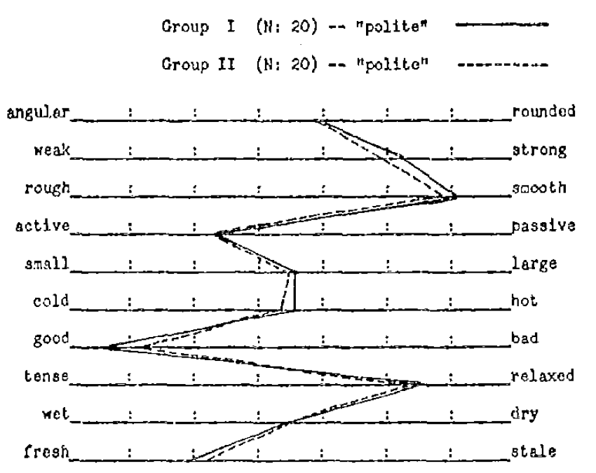] - Stimulus: One word, in this case *polite* - Response: Ratings of each participant for the word in relation to adjectives --- ## Semantic differential example: fonts .center[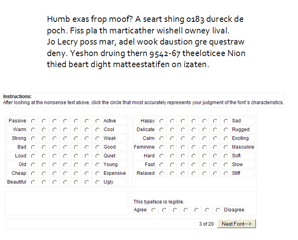] --- .center[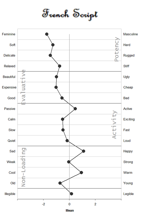] --- ## Dimensionality reduction: Factor analysis .center[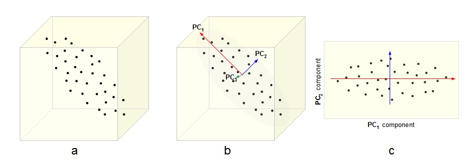] - The N-dimensional cloud of (average) ratings of words is processed with factor analysis - Each factor is a vector in the N-dimensional space. Factors are orthogonal - Factors are ordered such that the first one has the most variance - The result is a smaller set of dimensions that represents the ratings of words to certain extent (explained variance) --- # Three dimensions of meaning .pull-left[.center[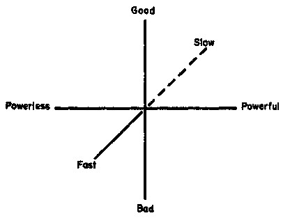]] .pull-right[ The dimensions of the Semantic Differential (EPA): - **Evaluation:** good, desirable -- bad, undesirable - **Potency:** strong, powerful -- weak, powerless - **Activation:** active, fast -- passive, slow] - Evaluation has the most variance, i.e is the most explanatory - Potency and Activation have similar explanatory level below Evaluation --- # Word embeddings ## 1. The semantic differential ## *2. Word embeddings* --- layout: true <div class="my-footer"><span>Speech and Language Processing. Daniel Jurafsky & James H. Martin. (2023)</span></div> --- # Documents as vectors  - Remember bag of words: term frequency counts ignoring order - Example just for four words in four books as documents - Here, each book is represented by a four-dimensional vector (vertical here) [Speech and Language Processing. Daniel Jurafsky & James H. Martin. (2023)](https://web.stanford.edu/~jurafsky/slp3/6.pdf) --- # Documents as vectors .center[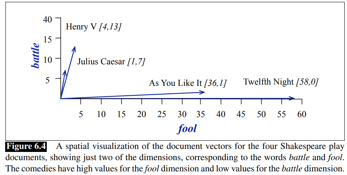] --- # Measuring similarity The similarity between the content of two documents can be measured with the cosine similarity of their vector representations: `$$sim(u,v) = cos(\theta) = \frac{u\cdot v}{\|u\| \|v\|} = \frac{\sum^n_{i=1}{u_iv_i}}{ \sqrt{\sum^n_{i=1} u_i^2} \sqrt{\sum^n_{i=1} v_i^2}}$$` `$$sim(d_1, d_2) = \frac{1*0 + 114*80 + 36 * 58 + 20 * 15}{\sqrt{1+114^2+36^2+20^2} \sqrt{80^2+58^2+15^2}} \sim 0.95$$` - `\(d_1\)`: As You Like It - `\(d_2\)`: Twelfth Night --- # Cosine similarity example .center[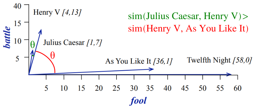] --- # Words as vectors .center[] - Instead of looking at document vectors, we can use word vectors - These vectors can approximate the meaning similarity between words - `\(sim(fool, wit) \sim 0.93\)` - `\(sim(fool, battle) \sim 0.09\)` - *fool* is not a synonym of *wit*, but its meaning is closer to *wit* than to *battle* --- ## Language sparsness and the curse of dimensionality .pull-left[ - Human languages have lots of different words - Heap's law: Vocabulary size grows (sublinearly) with corpus size - More documents, more words - Word and document matrices become too sparse - Hard to do statistics or train models when the vast majority of variables are zeroes - Larger corpora might not exist! ] .pull-right[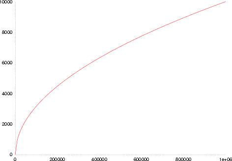 Number of distinct words (vocabulary size) versus corpus size (in tokens)] --- # Latent Semantic Analysis - Aim of LSA: making word and document vectors denser (less dimensions) - Idea: Singular Value Decomposition of word-document matrix - Problem: Very computationally intensive as soon as matrix gets large .center[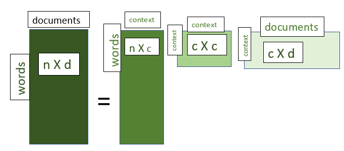] https://www.geeksforgeeks.org/latent-semantic-analysis/ --- # Distributed representations **The distributional hypothesis: Words that occur in similar contexts tend to have similar meanings** -- "You Shall Know a Word by the Company It Keeps" .center[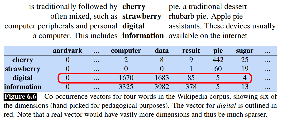] --- ## Self-supervision: Continuous Bag Of Words - Idea: training a model to predict words from their context: .center[the quick brown fox ... over the lazy dog] - Self-supervision: train it with corpus, without annotations - Represent each word `\(w\)` with a vector `\(\mu_{w}\)` in a lower-dimensional space compared to the word-document matrix (50-700 dimensions) - Fit the values of `\(\mu_w\)` with self-supervision such that: $$ argmax_{\mu_w} = \frac{exp(\mu_w \cdot \vec{v})}{\sum_j exp(\mu_j \cdot \vec{v})} $$ where `\(\vec{v}\)` is the mean vector for the words in the context and `\(j\)` iterates over the words in the language --- layout: true <div class="my-footer"><span>David Garcia - Social Data Science</span></div> --- .pull-left[ # ML Warning In this lecture we focus on applications, not development We will gloss over details, see references and related courses to learn more ] .pull-right[] --- # Word embeddings - After fitting, the resulting `\(\mu_w\)` are called **word embeddings** - Also called word representations: `\(R(w)\)` - Operating on embeddings space allow us to extract dimensions of meaning or compute analogies: .center[] --- # Word embeddings in practice You don't need to fit your own word embeddings model, several alternatives exist that are already trained: - word2vec [(Mikolov, Chen, Corrado, and Dean, 2013)](https://arxiv.org/abs/1301.3781) - Developed by Google - trained against Wikipedia - Based on CBOW and Skipgrams (predict context from word) - GloVe [(Pennington, Socher, Manning, 2014)](https://aclanthology.org/D14-1162/) - "global" embeddings using a larger definition of context - Developed by Stanford NLP group, similar to word2vec - fastText [(Bojanowski, Grave, Joulin, Mikolov, 2017)](https://arxiv.org/abs/1607.04606) - Developed by Facebook - trained against Wikipedia in many languages - Uses character-level tokenization: it can embed new words based on how they are written (e.g. composite words from the embeddings of lemmas) --- # Distributed Dictionary Representation .center[] [Dictionaries and distributions: Combining expert knowledge and large scale textual data content analysis. J. Garten, J. Hoover, K. Johnson, R. Boghrati, C. Iskiwitch & M. Dehghani. Behavior Research Methods (2018)](https://link.springer.com/article/10.3758/s13428-017-0875-9) --- # Distributed Dictionary Representation .center[] - Two tests: predicting if movie reviews are positive or negative and identifying moral foundations in tweets - DDR outperforms word counting and performs best when applied on a smaller dictionary - larger dictionaries is not better in this case