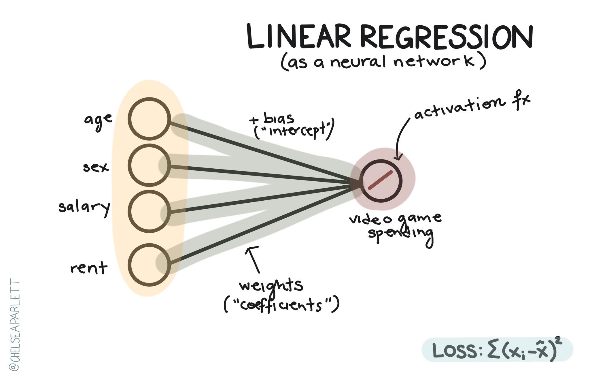
class: center, middle, inverse, title-slide .title[ # Linear Regression ] .author[ ### David Garcia <br><br> <em>ETH Zurich, Chair of Systems Design</em> ] .date[ ### Social Data Science ] --- layout: true <div class="my-footer"><span>David Garcia - Social Data Science - ETH Zurich, Chair of Systems Design</span></div> --- # Linear Regression Regression models formalize an equation in which one numeric variable `\(Y\)` is formulated as a linear function of other variables `\(X_1\)`, `\(X_2\)`, `\(X_3\)`, etc: <center> `\(Y = a + b_1 X_1 + b_2 X_2 + b_3 X_3 ... + \epsilon\)` </center> - `\(Y\)` is called the dependent variable - `\(X_1\)`, `\(X_2\)`, `\(X_3\)`, etc are called independent variables - `\(a\)` is the intercept, which measures the expected value of `\(Y\)` that does not depend on the dependent variables - `\(b_1\)`, `\(b_2\)`, `\(b_3\)`, etc are called the slopes or the coefficients - `\(\epsilon\)` are the residuals, the errors of the equation in the data ---  --- # Example: FOI vs GDP <img src="LinearRegression_Slides_files/figure-html/unnamed-chunk-1-1.png" style="display: block; margin: auto;" /> --- # Regression residuals Residuals ( `\(\epsilon\)` ) are the differences in between the empirical values `\(Y_i\)` and their fitted values `\(\hat Y_i\)`. <img src="LinearRegression_Slides_files/figure-html/unnamed-chunk-2-1.png" style="display: block; margin: auto;" /> --- # Ordinary Least Squares (OLS) **Fitting** a regression model is the task of finding the values of the coefficients ( `\(a\)`, `\(b_1\)`, `\(b_2\)`, etc ) in a way that reduce a way to aggregate the residuals of the model. One approach is called Residual Sum of Squares (RSS), which aggregates residuals as: <center> `\(RSS = \sum_i (\hat Y_i - Y_i)^2\)` </center> The Ordinary Least Squares method (OLS) looks for the values of coefficients that minimize the RSS. This way, you can think about the OLS result as the line that minimizes the sum of squared lengths of the vertical lines in the figure above. --- # Regression in R The lm() function in R fits a linear regression model with OLS. You have to specify the *formula* of your regression model. For the case of one independent variable, a formula reads like this: ```r DependentVariable ∼ IndependentVariable ``` If you print the result of lm(), you will see the best fitting values for the coefficients (intercept and slope): ```r model <- lm(GDP~FOI, df) model$coefficients ``` ``` ## (Intercept) FOI ## -4309.223 54631.170 ``` --- # Goodness of fit A way to measure the quality of a model fit this is to calculate the proportion of variance of the dependent variable ( `\(V[Y]\)` ) that is explained by the model. We can do this by comparing the variance of residuals ( `\(V[\epsilon]\)` ) to the variance of `\(Y\)`. This is captured by the coefficient of determination, also known as `\(R^2\)`: <center> `\(R^2 = 1 − \frac{V[\epsilon]}{V[Y]}\)` </center> For our model example: ```r 1-var(residuals(model))/var(df$GDP) ``` ``` ## [1] 0.4432583 ``` --- # Multiple regression You can specify models with more than one independent variable by using "+": ```r DependentVariable ∼ IndependentVariable1 + IndependentVariable2 + IndependentVariable3 ``` If we wanted to fit a model of GDP as a linear combination of the FOI and the internet penetration in countries, we can do it as follows: ```r model2 <- lm(GDP~FOI+IT.NET.USER.ZS, df) model2$coefficients ``` ``` ## (Intercept) FOI IT.NET.USER.ZS ## -16154.2983 20528.8273 539.8481 ``` ```r summary(model2)$r.squared ``` ``` ## [1] 0.8140538 ``` --- # Regression diagnostics ```r hist(residuals(model), main="", cex.lab=1.5, cex.axis=2) ``` <img src="LinearRegression_Slides_files/figure-html/unnamed-chunk-8-1.png" style="display: block; margin: auto;" /> --- # Regression diagnostics ```r plot(predict(model), residuals(model), cex.lab=1.5, cex.axis=2) ``` <img src="LinearRegression_Slides_files/figure-html/unnamed-chunk-9-1.png" style="display: block; margin: auto;" /> --- <center>  </center>